Computer Vision Coursework

UCI CS 116 · Winter 2025 · Individual coursework (six assignments)

Six assignments, from bilinear interpolation to panorama stitching, texture quilting, HOG object detection, and sampling and editing with a pretrained diffusion model

Stack

Python, NumPy, SciPy (ndimage, interpolate), Matplotlib, scikit-image, PyTorch, Jupyter, DeepFloyd IF (pretrained)

Goal and outcome

The course was taught through notebook assignments. Each notebook gave the problem, scaffolding and some test stubs; I implemented the algorithms, wrote test cases, ran the experiments and wrote the discussion. The six assignments:

  • NumPy and Matplotlib warm-up: loading images, sub-regions, histograms, threshold masks.
  • Interpolation: linear (1D) and bilinear (2D) interpolation to upsample and warp images.
  • Panorama mosaics: point correspondences, homographies by least squares, warping and feathered blending (Problem 1).
  • Texture quilting: a dynamic-programming minimum-cost seam that stitches sampled patches into new texture (Problem 2).
  • Object detection: image gradients and HOG features, templates learned from positive and negative crops, detection with non-maximum suppression; then the same detector on pretrained CNN features.
  • Diffusion: around a pretrained DeepFloyd IF model, the forward noising process, one-step and iterative denoising, classifier-free guidance, image-to-image translation, sketch-to-image and inpainting.

Every assignment runs end to end in its notebook with the results saved; the figures on this page come from those notebooks.

My role

Individual work. The split below follows what each notebook marks as provided versus left for the student.

Written by me

  • Interpolation: linear_interpolate, bilinear_interpolate and their tests
  • Panorama: get_correspondences (the point-picking loop), compute_homography, apply_homography, warp_images, blend_images and the result figures
  • Quilting: shortest_path, stitch, synth_quilt, the parameter experiments and two textures of my choice
  • Detection: mygradient, hog, detect, learn_template, the face and traffic-sign experiments, learn_template_cnn and detect_cnn
  • Diffusion: forwardnoise, one-step denoising, add_variance, iterative_denoise, iterative_denoise_cfg, image2image, inpaint and the experiments

Provided by the course

  • Notebook templates, problem statements, some plotting code and test stubs
  • selectpoints.py (click-to-select UI) and hogvis.py (HOG visualization)
  • quilt_demo, sample_tiles and topkmatch (tile sampling and candidate matching)
  • The pretrained CNN feature extractor (extractfeatures); the pretrained DeepFloyd IF model, its noise schedule and precomputed text embeddings
  • Data: the atrium and window photo sets, the rock-wall texture, face images and the diffusion test image

Technical problems

Problem 1: Aligning and blending photos into one panorama

Problem
Photos taken by rotating a camera about one point can be aligned with a homography, but two things go wrong: warped photos land at negative or out-of-frame coordinates, and pasting them on top of each other leaves visible seams where exposure and alignment differ slightly.
What I did
  • Estimate each homography by linear least squares: two equations per point pair, h33 fixed to 1, solved with np.linalg.lstsq. For the two course sets I clicked 16 pairs per photo (the minimum is 4).
  • Size the output canvas by warping each photo's four corners into the base photo's frame and taking the bounding box; then map every pixel through its homography and resample onto the canvas grid with SciPy's griddata.
  • Blend with feathered alpha masks: each photo's weight is its distance transform from the photo's edge, clipped at 55 px, then normalized so overlapping weights sum to 1; pixels no photo covers stay black.
Why this approach
Least squares over more than four pairs averages out click error instead of fitting a few bad clicks exactly. Distance-transform weights fall to zero at each photo's border, so the change from one photo to the next spreads across the overlap rather than happening at a hard edge; clipping at 55 px confines that transition to a band near each edge.

Five campus photos taken by rotating the camera from one spotOpen full-size image
Input: five course-provided photos taken by rotating the camera about one point.
Five normalized alpha masks, white where weight is high, fading toward each photo's edgeOpen full-size image
My feathered alpha masks after normalization (white = high weight): each fades toward its photo's edge, so overlaps blend gradually.
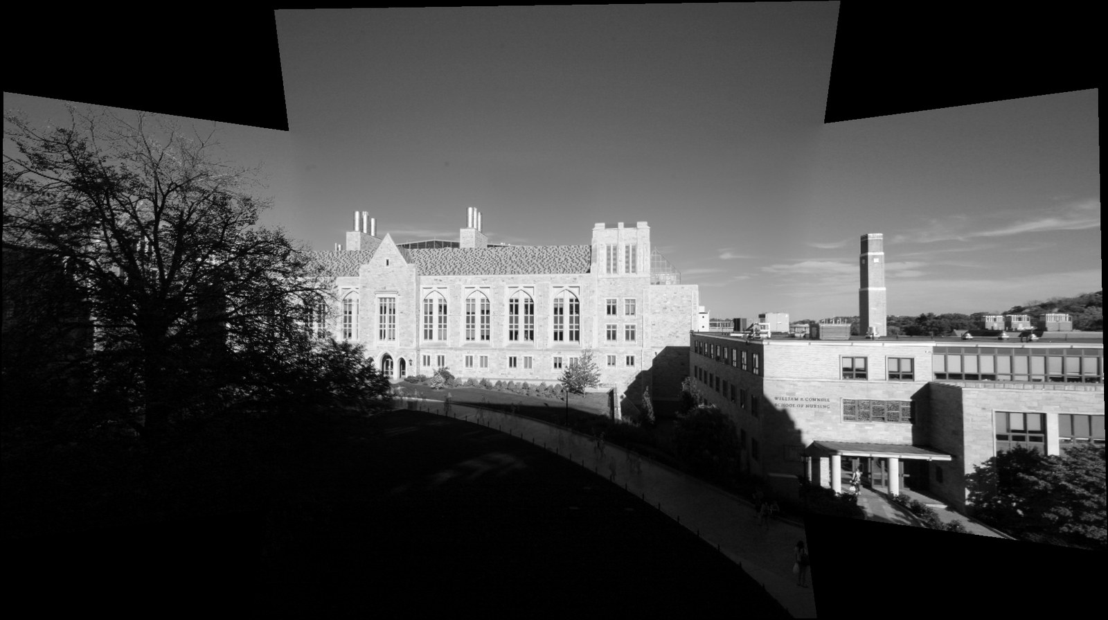
The five photos stitched into one wide panoramaOpen full-size image
Output: the five photos as one mosaic (re-rendered from my notebook code and saved point clicks).
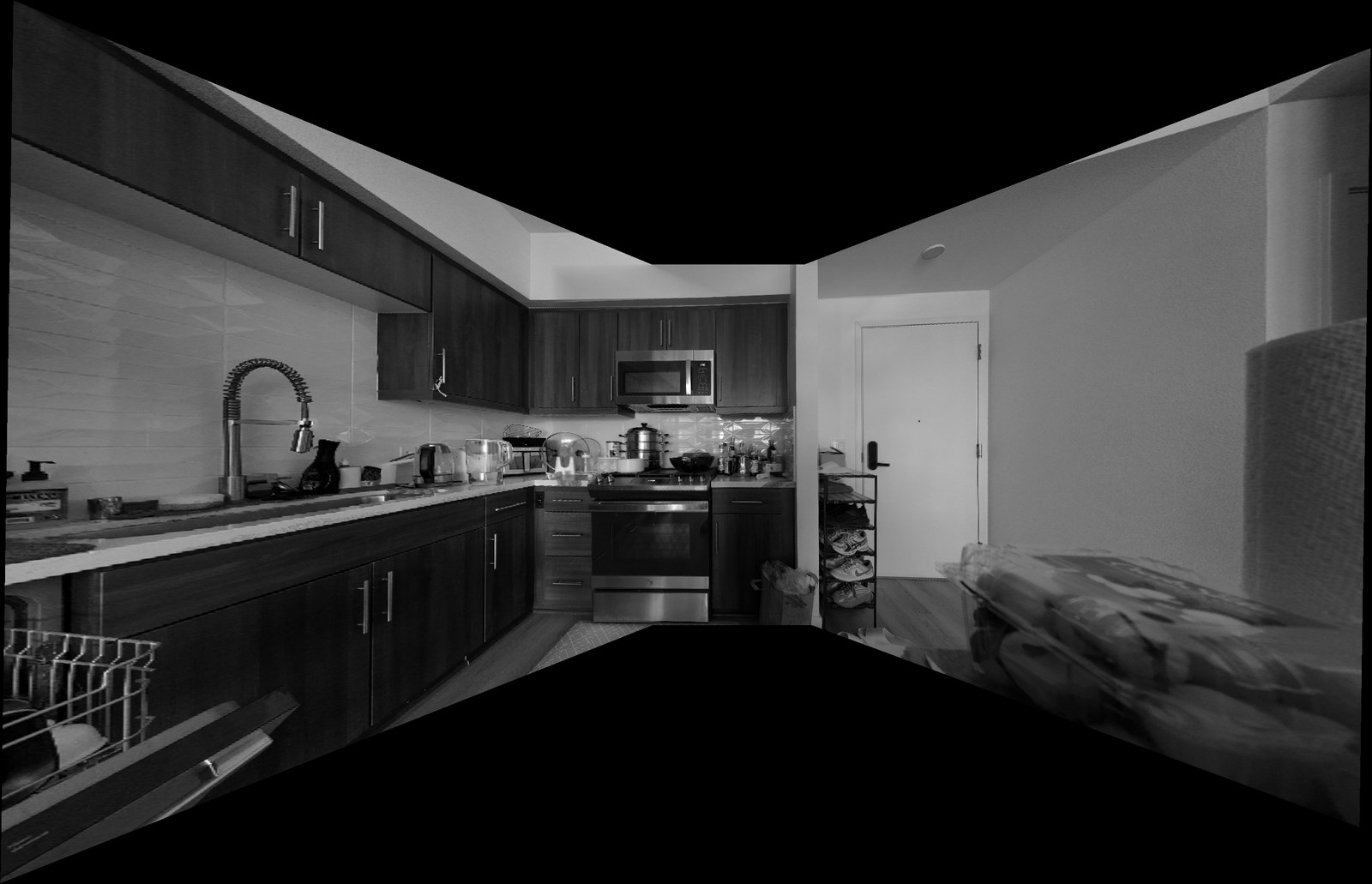
A kitchen panorama stitched from three of my own photosOpen full-size image
Three photos I took of a kitchen, stitched with the middle photo as the base and 8 point pairs per side photo (also re-rendered).

Problem 2: Stitching texture patches along the least visible seam

Problem
Texture quilting builds a large texture by tiling patches sampled from a small example. Neighboring patches never line up exactly, so cutting the overlap with a straight line leaves an obvious grid of edges.
What I did
  • In each overlap strip, use the per-pixel absolute difference between the two patches as a cost, and find the top-to-bottom path of least total cost that moves at most one column left or right per row.
  • Solve it with dynamic programming: M[i, j] = cost[i, j] + min(M[i−1, j−1], M[i−1, j], M[i−1, j+1]). Each row is computed at once by stacking the previous row shifted left and right (padded with ∞) and taking the min and argmin; the path is then traced back from the cheapest end.
  • Stitch along that seam: pixels left of the path come from the left patch, the rest from the right one. Rows of tiles are built left to right, then the rows are stitched top to bottom by transposing.
Why this approach
A cut through pixels where the two patches already agree is hard to see. The dynamic program finds the globally cheapest seam in O(H·W) for an H×W strip, while a greedy row-by-row choice can miss it; one of my test cases is built so that greedy search fails and the DP doesn't.
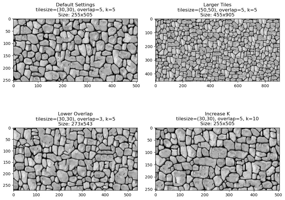
Four rock-wall textures synthesized with default settings, larger tiles, smaller overlap and more candidatesOpen full-size image
Rock-wall texture (course-provided example) synthesized by my quilting code under four settings: default, larger tiles, smaller overlap and more candidate tiles (k).

Results and verification

Eight stages of iterative denoising, from pure noise to a street sceneOpen full-size image
Iterative denoising from pure noise with my iterative_denoise and the pretrained DeepFloyd IF model (64×64 stage-1 output, prompt “a high quality photo”), from t = 990 to the final image.
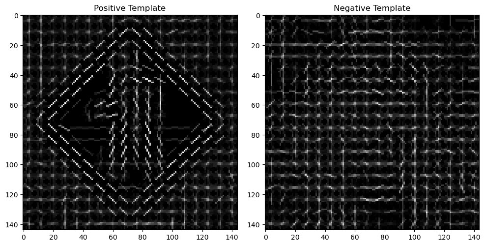
The average HOG templates for positive and negative traffic-sign cropsOpen full-size image
HOG templates learned for traffic signs: the average over five positive crops (left) and five negative crops (right). Detection correlates their difference with the image's HOG map.
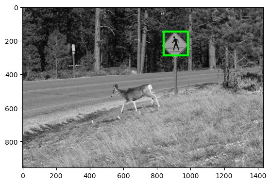
A deer by a road, with the detection box on a pedestrian signOpen full-size image
The top detection on one of the test photos I chose lands on the pedestrian sign; it did on all three test photos.
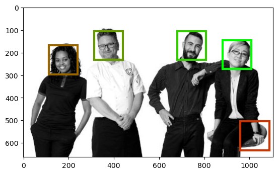
A group photo of four people, with boxes on the four faces and a fifth box on a handOpen full-size image
HOG face detection on a course-provided group photo (top 5, green = highest score, red = lowest): the four faces rank first; the fifth box lands on a hand.
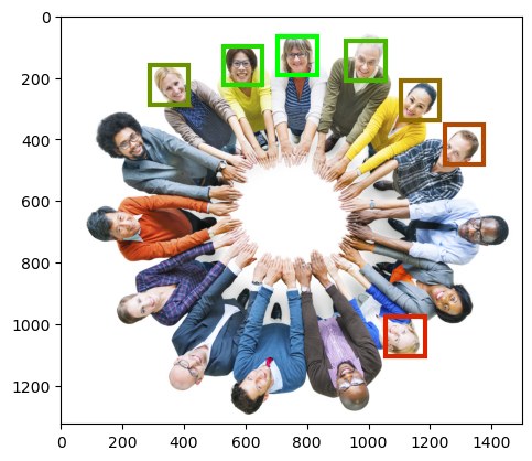
People in a circle seen from above, with all seven boxes on facesOpen full-size image
The same detector on pretrained CNN features, with faces arranged in a circle (top 7): all seven boxes are on faces, including an upside-down one at the bottom right.
  • Quilting parameter study (my written analysis in the notebook): larger tiles (50 px) kept more of the original stone structure; a smaller overlap (3 px) made seams more visible because there are fewer pixels to route a seam through; more candidates (k = 10) gave more variety.
  • Detection: the sign template, taking only the top-scoring detection per photo, landed on the sign in all three test photos. On face images, switching to CNN features was clearly more accurate than HOG and still found faces arranged in a circle, which I attributed to more robustness to variation such as rotation.
  • How it was checked: each notebook has test cells (interpolation results against hand-computed values with assert_allclose, homography round trips through H and H⁻¹, and hand-built cost arrays with known shortest paths), plus saved visual results.

Limitations

  • Panorama correspondences are clicked by hand, with no automatic feature matching or RANSAC, so alignment depends on click accuracy; photos are downsampled to 876×584 and processed in grayscale.
  • The HOG detector uses one fixed-size template, so it only finds objects near the training scale and orientation.
  • The diffusion work uses a pretrained model: I wrote the sampling and editing loops around it, not the model or its training.
  • These are guided course assignments: the problem setup, scaffolding and data came from the course.

Evidence

No public links: these are graded assignments that may be reused, so the notebooks and code stay private. Every figure on this page was exported from my submitted notebooks.